How To Use VLookUP in Excel! Best Techywired’s Guide

The typical user doesn’t use many useful features and tools in Microsoft Excel 2016. However, look at VLOOKUP in excel if you notice yourself always looking in the same table for information. VLOOKUP, an abbreviation for “vertical lookup,” is a powerful way to rapidly find records corresponding to a given value using vertically aligned tables.

For instance, if you have a product’s name and need to find out how much it costs quickly, you may use Excel’s VLOOKUP function. Setting up VLOOKUP might seem daunting to a first-time Excel user, but it’s rather simple. Please refer to our comprehensive guide if you need help with VLOOKUP in Excel.

It’s safe to say that VLOOKUP in Excel features the greatest notoriety, for better or worse. VLOOKUP, on the plus side, straightforwardly does a valuable task. Watching VLOOKUP search a table, locate a match, and deliver a good result is gratifying, especially for first-time users. The ability to effectively utilize VLOOKUP in excel marks the transition from Excel novice to seasoned pro.

VLOOKUP’s shortcomings and risky defaults are major drawbacks. VLOOKUP requires a whole table with lookup values in the first column, unlike INDEX and MATCH (or XLOOKUP). As a result, VLOOKUP in excel becomes cumbersome when dealing with several criteria. VLOOKUP also tends to provide inaccurate results due to its default matching strategy. Not to worry. Learning the fundamentals of VLOOKUP in excel is crucial if you want to use it effectively. The next paragraphs will provide you with an in-depth summary.

Microsoft Excel may be a time-consuming nightmare when coordinating large amounts of data. Having to compare data from various spreadsheets might add to the stress. To move cells manually using paste and copy should be avoided at all costs. Fortunately, that is not the case. If you have access to Microsoft Excel, the VLOOKUP in excel tool may assist in automating this process.

I realize the term “VLOOKUP function” conjures images of the most convoluted, geekiest, most complex concept. However, after reading this post, you won’t know how you managed without it in Excel.

The VLOOKUP in Excel is more intuitive than you would believe. Moreover, it is a potent analytical tool that should not be missing from your toolkit.

How does VLOOKUP in Excel work?

The abbreviation “VLOOKUP” means “vertical lookup.” This is accomplished in Excel by utilizing the spreadsheet’s columns and a column’s unique identifier as the foundation for a vertical search over the spreadsheet’s data. The information you’re looking for must be presented in a vertical list format regardless of storage location.

For some reason, the formula is constantly looking to the right.

Excel’s VLOOKUP function is used to find updated information in a separate workbook corresponding to previously entered information in the active workbook. When doing this search using VLOOKUP, the function always scans the area to the right of the current cell for updated information.

For instance, if you have a vertical list of names in one spreadsheet and a random assortment of email addresses in another, you may use VLOOKUP in excel to obtain the email addresses in the order they appear in the first spreadsheet. If you want Excel to locate such emails, you must put them in the column to the right of the names in the second spreadsheet.

The formula needs a unique identifier to retrieve data.

The secret to how VLOOKUP in excel works? Unique identifiers.

Unlike any other information in your data sets, a “unique identifier” cannot be duplicated. Product numbers, stock-keeping units (SKUs), and client information qualify as unique identifiers.

Now that we’ve seen how the VLOOKUP works let’s look at another example!

VLOOKUP In Excel Example

The VLOOKUP in excel function is shown in the following video as it links emails (from a secondary data source) with their relevant information on a third sheet.

The following is an example of a VLOOKUP in Excel function:

VLOOKUP(lookup_value , table_array , col_index_num , range_lookup)

Here, we’ll go through the processes needed to properly fill these fields with the MRR for each client, replacing the customer names.

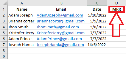
1. Identify a column of cells you’d like to fill with new data.

Remember that your goal is to copy information from another page into this one. To do this, type a descriptive title in the top cell of the column adjacent to the columns you’re interested in learning more about, such as “MRR” (monthly recurring revenue). The information you’re retrieving will be entered into this new column.

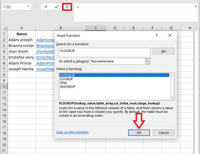
2. Select ‘Function’ (Fx) > VLOOKUP in Excel and insert this formula into your highlighted cell.

Look for a little function icon in the shape of a script labeled Fx in a text bar spreadsheet. To use it, choose the column heading and then click the blank cell that appears just underneath it. To the right of the screen, you’ll see a box labeled Formula Builder or Insert Function.

In the Formula Builder, look for the “VLOOKUP” option and click on it. To begin creating your VLOOKUP in excel, click OK or Insert Function. You should now see “=VLOOKUP()” in the selected cell of the spreadsheet.

Manually inputting the formula into a call involves typing the bolded language above into the relevant cell.

After typing =VLOOKUP in excel into the first empty cell, you must input four different conditions into the formula. By providing Excel with these details, you may direct it to the specific location and kind of information you want.

For more Similar articles, you can visit Techywired.

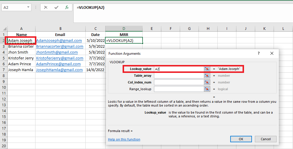
3. Enter the lookup value for which you want to retrieve new data.

The first criterion is the lookup value or the cell or range of cells whose contents you want Excel to locate and get based on a set of criteria you provide. Simply input the value you’re looking to match by clicking on the cell containing it. As you can see above, in our case, it is located in cell A2. Since the MRR for the client whose name is A2 is in D2, here is where you’ll begin entering your new information.

The key is to remember that your lookup value may be anything at all (text, numbers, URLs, etc.). The function will provide the desired information if the value you enter matches the one in the referencing spreadsheet, which we will cover in the next section.

4. Enter the table array of the spreadsheet where your desired data is located.

Copy and paste the format in the screenshot above into the “table array” box, then input the range of cells you want to search and the page where these cells are placed. If you see an item like the one above, it signifies the information we need is in a spreadsheet labeled “Pages,” which may be located between columns B and K.

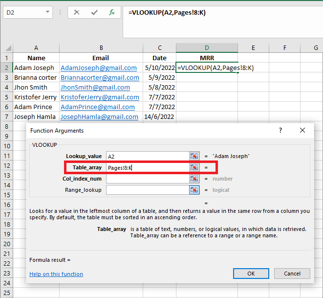
The data sheet must already exist in the open Excel workbook. This implies that your data might be located in a separate table of cells anywhere in the current spreadsheet or in a separate spreadsheet attached at the bottom of your worksheet, as demonstrated in the following example.

If you want to access information in cells C7 and L18 on “Sheet2,” you would create the table array entry “Sheet2!C7:k87.”

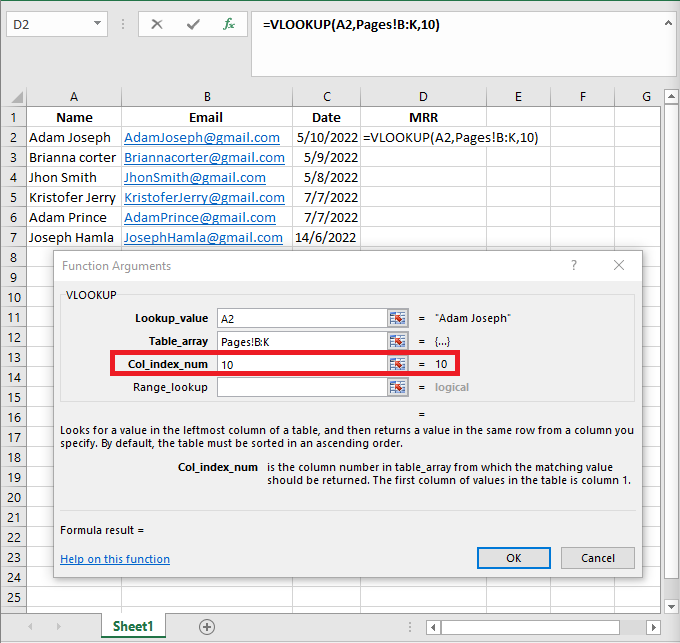
5. Enter the column number of the data you want Excel to return.

Insert the “column index number” for the table array you want to search under the table array field. If the numbers you’re looking for are in Column K, but you’re only interested in Columns B through K (which would be put as “B: K” in the “table array” field), then you would enter “10” in the “column index number” field.

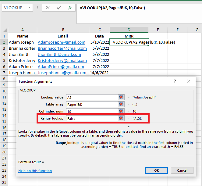
6. Enter your range lookup to find an exact or approximate match of your lookup value.

When dealing with monthly income as we are, it is essential to identify precise matches in the table you are going through. To accomplish this, in the range lookup box, type “FALSE.” This informs Excel that you only care about the hard numbers for each sales contact’s income.

In response to your critical inquiry, Excel may be instructed to settle for a close rather than an exact match. To do so, replace the text in the fourth field with TRUE.

If you tell VLOOkUP in excel to find the closest match rather than an exact one, it will seek values similar to the one you’re looking for. For example, if you’re searching for information on a set of website links and some of those links start with “https://,” it could be prudent to hunt for a close match in case some of the links in your set don’t start with that prefix. In this manner, your VLOOKUP in excel calculation won’t fail with an error if Excel can’t detect the first text tag in the link.

7. Click ‘Done’ (or ‘Enter’) and fill in your new column.

After completing the “range lookup” box, click “Done” (or “Enter,” depending on your version of Excel) to formally bring in the numbers you want into your new column from Step 1. Your first cell will be filled in this way. You may consult the other spreadsheet if you want to double-check that this is the right number.

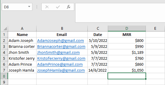
If this is the case, choose the first cell in the new column to be filled, then click the small square in the cell’s lower right corner. This will cause the other cells in the new column to be filled with the following values. Done! You should now see all of your values.

Vlookup: a Powerful Marketing Tool

To gain a complete view of lead creation, marketers need to examine data from many different sources (and more). Since the VLOOKUP feature is built into Microsoft Excel, it is the ideal program for doing this precisely and in large quantities.

FAQs